2024-28-05 Tidy Tuesday

Lisa’s Vegetable Garden Data

Author

Griffin Judy

Published

May 28, 2024

Introduction

Tidy Tuesday is a weekly data project shared on the Tidy Tuesday Github. In this article, I explore the data and reflect on my first Tidy Tuesday.

Intake and Exploring

The tidyverse package is extremely useful in assisting with data manipulation, processing, and visualization.

Code

library(tidyverse)
options(dplyr.summarise.inform = FALSE)

The first step to any data analysis is loading the data and reviewing it. Thankfully, the Tidy Tuesday Github shows how to load the data and the data dictionary. A brief look at each table can be found in Appendix 1.1.

Reading the data

#Read in the data 
spending_2020 <- readr::read_csv('https://raw.githubusercontent.com/rfordatascience/tidytuesday/master/data/2024/2024-05-28/spending_2020.csv')
spending_2021 <- readr::read_csv('https://raw.githubusercontent.com/rfordatascience/tidytuesday/master/data/2024/2024-05-28/spending_2021.csv')

This dataset includes six tables: spending data for 2020, spending data for 2021, planting data for 2020, planting data for 2021, harvest data for 2020, and harvest data for 2021. This article will examine the spending data.

Results and Plots

Since the dataset is comprised three paired sets (2020 and 2021), there may be interesting relationships and descriptive analytics present.

Code

#combining both spending years for easier visualizations
#remove a column in the 2020 data that is not present in 2021, will not be used
spend_2020 <- spending_2020[,-4] 
spend_2020 <- mutate(spend_2020,year = 2020)
spend_2021 <- mutate(spending_2021,year = 2021)
SPENDING <- rbind(spend_2020,spend_2021)

Price without tax and price with tax is supplied. The items may have a different tax rate.

Code

SPENDING |> #dataset
  #group purchases by which vegetable they are
  group_by(vegetable) |> 
  #remove vegetables recieve for no cost
  filter(price > 0 ) |> 
  #taxrate = taxed_price/untaxted_price
  summarise(taxrate = mean(price_with_tax/price))|> 
  reframe(tax_rate_range = range(taxrate))

# A tibble: 2 × 1
  tax_rate_range
           <dbl>
1           1.08
2           1.08

All items that were not received for free have that same tax rate. How did the price of items change year-over-year? The difference in average price needs to be found.

Code

V_PRICE <- SPENDING |> #dataset
  #group purchases by which vegetable they are
  group_by(vegetable,year) |>
  summarise(mean_price = mean(price)) 

#gives where the veggies appear in 1 year (n=1) or both (n=2)
V_COUNT <- V_PRICE |>
  count(V_PRICE$vegetable)

#which veggies that were present both years
V_TWO <- V_COUNT[which(V_COUNT$n != 1),]

#veggies that were present both years and prices
V_TWO_PRICE <- left_join(V_TWO,V_PRICE)

#returns the veggies, ordered by year
V_TWO_PLOT <- V_TWO_PRICE |>
  group_by(vegetable) |>
  arrange(desc(year)) |>
  # 2021 price - 2020 price
  mutate(price_diff = mean_price - lag(mean_price)) |>
  filter(!is.na(price_diff)) |>
  arrange(desc(price_diff))

#printing the table
knitr::kable(V_TWO_PLOT[,c(1,6)])

vegetable	price_diff
dill	0.2500000
basil	0.1250000
kale	0.0000000
swiss chard	0.0000000
spinach	-0.0100000
beets	-0.1000000
lettuce	-0.2983333
carrots	-0.4800000

Formatting and a plot will make the the differences easier to visualize.

Code

p <- ggplot(V_TWO_PLOT, aes(x = reorder(vegetable, price_diff), y = price_diff)) +
  theme_minimal() +
  guides(fill="none") + #no legend
  geom_col(position = "dodge") + #bars will not touch
  #vjust is set to value based on value of bars for consistency
  theme(axis.text.x = element_text(vjust = .7,angle = 45,)) + 
  geom_text(aes(label = format(round(price_diff, 2), nsmall=2)),
            vjust = ifelse(V_TWO_PLOT$price_diff < 0, 1, -.3)) +
  labs(title = "Difference in Avg Price of Vegetables, 2020-2021",
       x = "Vegetables",
       y = "Price Difference")
p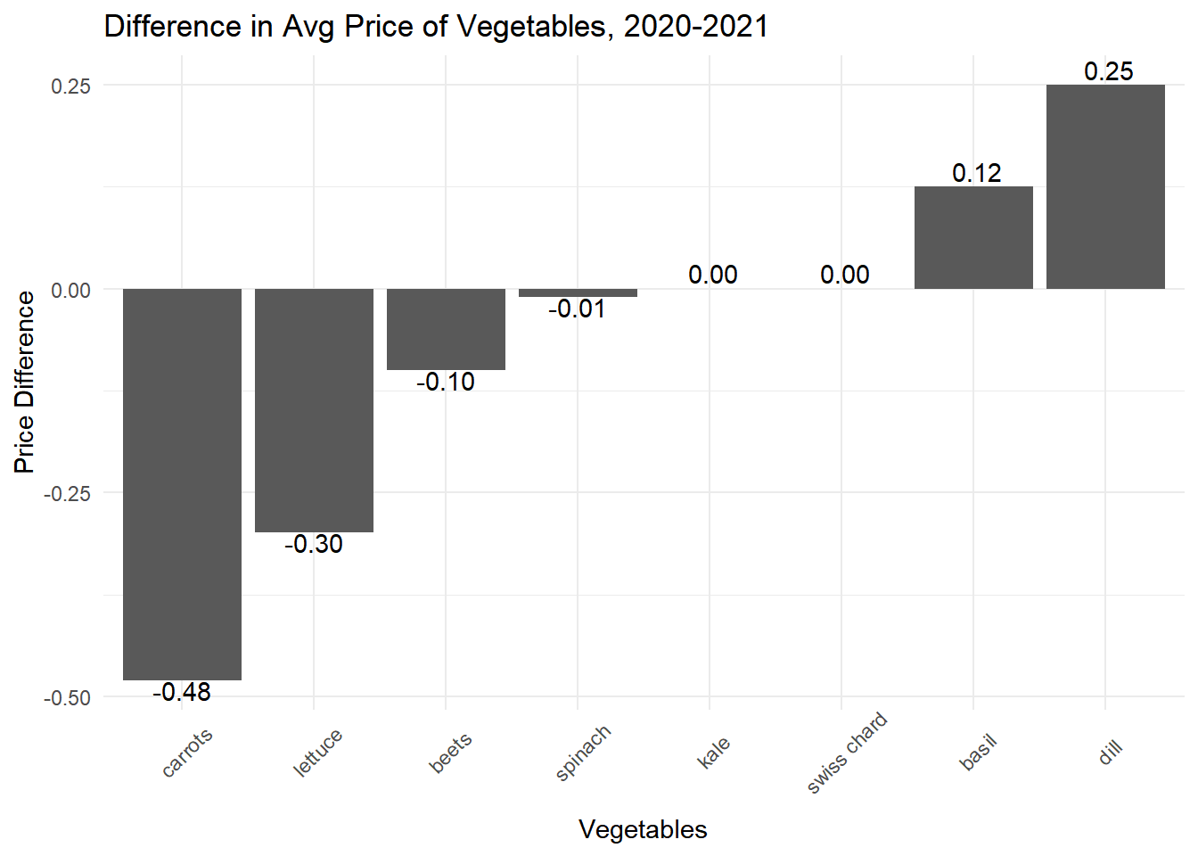

More vegetables reduced in price than increased in price.

Reflection

This week is my first Tidy Tuesday, and I enjoyed it! I started late, so I was not able to get as far as I wanted. I spent more time adjusting Quarto html/web publishing than performing analysis, but I believe I have a better understanding of the workflow. I look forward to next week!

Appendix

1.1 Brief Look at Each Table

Brief look at each table

knitr::kable(head(spending_2020),caption = "spending_2020")

spending_2020
vegetable	variety	brand	eggplant_item_number	price	price_with_tax
beans	Bush Bush Slender	Renee’s Garden	2156	2.79	3.009713
beans	Chinese Red Noodle	Baker Creek	2138	3.00	3.236250
beans	Classic Slenderette	Renee’s Garden	2157	2.99	3.225462
beets	Gourmet Golden	Renee’s Garden	1018	3.19	3.441212
beets	Sweet Merlin	Renee’s Garden	2114	2.99	3.225462
broccoli	Yod Fah	Baker Creek	37097	3.00	3.236250

Brief look at each table

knitr::kable(head(spending_2021),caption = "spending_2021")

spending_2021
vegetable	variety	brand	price	price_with_tax
cabbage	early jersey wakefield	Seed Savers	2.99	3.225462
kale	heirloom lacinto	Renee’s Garden	2.79	3.009713
basil	emily	Baker Creek	3.00	3.236250
basil	genovese	Seed Savers	3.25	3.505937
swiss chard	neon glow	Renee’s Garden	2.99	3.225462
lettuce	romaine jericho	Renee’s Garden	3.79	4.088463

1.2 All Code

All code on this page

library(tidyverse)
options(dplyr.summarise.inform = FALSE)

#read in the data
spending_2020 <- readr::read_csv('https://raw.githubusercontent.com/rfordatascience/tidytuesday/master/data/2024/2024-05-28/spending_2020.csv')
spending_2021 <- readr::read_csv('https://raw.githubusercontent.com/rfordatascience/tidytuesday/master/data/2024/2024-05-28/spending_2021.csv')

#combining both spending years for easier visualizations
#remove a column in the 2020 data that is not present in 2021, will not be used
spend_2020 <- spending_2020[,-4] 
spend_2020 <- mutate(spend_2020,year = 2020)
spend_2021 <- mutate(spending_2021,year = 2021)
SPENDING <- rbind(spend_2020,spend_2021)

SPENDING |> #dataset
  #group purchases by which vegetable they are
  group_by(vegetable) |> 
  #remove vegetables recieve for no cost
  filter(price > 0 ) |> 
  #taxrate = taxed_price/untaxted_price
  summarise(taxrate = mean(price_with_tax/price))|> 
  reframe(tax_rate_range = range(taxrate))

#| warning: false
V_PRICE <- SPENDING |> #dataset
  #group purchases by which vegetable they are
  group_by(vegetable,year) |>
  summarise(mean_price = mean(price)) 

#gives where the veggies appear in 1 year (n=1) or both (n=2)
V_COUNT <- V_PRICE |>
  count(V_PRICE$vegetable)

#which veggies that were present both years
V_TWO <- V_COUNT[which(V_COUNT$n != 1),]

#veggies that were present both years and prices
V_TWO_PRICE <- left_join(V_TWO,V_PRICE)

#returns the veggies, ordered by year
V_TWO_PLOT <- V_TWO_PRICE |>
  group_by(vegetable) |>
  arrange(desc(year)) |>
  # 2021 price - 2020 price
  mutate(price_diff = mean_price - lag(mean_price)) |>
  filter(!is.na(price_diff)) |>
  arrange(desc(price_diff))

#printing the table
knitr::kable(V_TWO_PLOT[,c(1,6)])

ggplot(V_TWO_PLOT, aes(x = reorder(vegetable, price_diff), y = price_diff)) +
  theme_minimal()+
  guides(fill="none")+
  geom_col(position = "dodge")+
  theme(axis.text.x = element_text(vjust = .7,angle = 45,)) + 
  geom_text(aes(label = format(round(price_diff, 2), nsmall=2)),
            vjust = ifelse(V_TWO_PLOT$price_diff < 0, 1, -.3))+
  labs(title = "Difference in Avg Price of Vegetables, 2020-2021",
       x = "Vegetables",
       y = "Price Difference")